Easy way for positioning data into uitable – Matlab

Matlab offers a simple way to display tabular data inside ower GUI’s. In this post I will show the simplest way to fill data inside the uitable. Using this way, it is possible to skip rows and columns to make the resulting table prettier

    %Create the main figure
    figure_object = figure;
    
    %Create the uitable with row and column names
    row_names = {'Subject 1', 'Subject 2', 'Subject 3' , 'Subject 4', '', 'Total'};
    col_names = {'Name', '', 'Variable 1', 'Variable 2', 'Variable 3', 'Variable 4'};
    
    table_object = uitable('Parent', f,...
        'Rowname', row_names,...
        'ColumnName', col_names,...
        'Position', [20, 20, 550, 150]);

    %Initiate table data structure
    nrows = 6;
    ncols = 6
    table_data = cell(nrows, ncols);

    %Fill the cells with subject names
    table_data(1:4) = {'Paul', 'Joseph', 'Mary', 'Carl'};

    %Fill the cells with some random values and skip one row
    %and one column
    table_data(1:6, 3) = {'10.23', '09.12', '12.67', '11.04', '', '43.06'};
    table_data(1:6, 4) = {'110.42', '67.09', '82.61', '101.04', '', '361.16'};
    table_data(1:6, 5) = {'0.45', '1.23', '0.54', '3.11', '', '5.33'};
    table_data(1:6, 6) = {'Yes', 'No', 'No', 'Yes', '', ''}

Resulting GUI

Bildschirmfoto 2015-07-05 um 12.45.07 vorm.

Curso de Matlab voltados para alunos da área de saúde e biologia

Estão abertas as inscriçōes para o CURSO DE INTRODUÇÃO AO MATLAB voltado aos alunos das áreas de saúde e biologia. Tal curso será realizado por quatro terças-feiras consecutivas na Sala A CAE HUCFF, da Universidade Federal do Rio de Janeiro, campus do Fundāo, tendo início no dia 10 de Março. Cada aula terá 4 horas de duraçāo, totalizando-se 16 horas.

curso_matlab.001

Ao longo do curso serāo abordados pontos fundamentais para programaçāo em Matlab e qualquer outra linguagem, como, por exemplo, tipos de variáveis, matrizes, vetores, controle de fluxo com laços for while, cláusulas if, else, end, construçōes de funçōes etc.
Além destes pontos, serāo apresentadas soluçōes para problemas presentes no dia-a-dia de pesquisadores. Abrangeremos temas como a abertura de arquivos, a manipulaçāo de planilhas em Excel, plot de figuras, processamento de sinais e estatísitca.

No último dia, todo o conhecimento adquirido será utilizado para construir programas com interface ao usuário, o que facilita muito a utilização por outros usuários e o programa que foi utilizado em seu Mestrado ou Doutorado pode ser um legado do laboratório que irá facilitar muito a vida de outros pesquisadores.

Exemplo de um programa com interface ao usuário desenvolvido em Matlab

Exemplo de um programa com interface ao usuário desenvolvido em Matlab.

Logo abaixo segue uma lista com os tópicos que serāo abordados no curso:

  • AULA 1- Carga horária 4h
    • O que é Programaçāo?
    • Por que Matlab?
    • Alternativas
      • Octave
      • FreeMat
      • SciLab
    • Introduçāo ao ambiente de trabalho
    • Hello World
    • Tipos de Variáveis
    • Comentários
    • Operadores
    • Controle de Fluxo
      • for
      • while
      • if
      • else
      • switch
    • Editor de Scripts e Funçōes
    • Boas Práticas
    • Definiçāo de funçōes
    • Exercícios em sala
    • Exercícios próxima aula
  • AULA 2 – Carga horária 4h
    • Funçōes Matemáticas
    • Vetores
    • Matrizes
    • Operaçōes com vetores e matrizez
    • Visualizaçāo
      • Plot
      • Subplot
      • Inteaçāo com gráficos
      • Plot 3D
    • Exercícios em sala
    • Exercícios próxima aula


  • AULA 3 – Carga horária 4h
    • Manipulaçāo de Arquivos
      • Leitura e Escrita em Arquivos
      • Aruivos Texto
      • CSV
      • Excel
    • Processamento de Sinais
      • Fourier
      • Filtros
      • Short Time Fourier Transform
      • Ajuste de Curvas
    • Estatística
      • Plot com barras de erro
      • Histogramas
      • Box-Plot
      • Comparaçāo de Médias
      • Correlaçāo
      • ANOVA
      • Teste de Normalidade
      • Integraçāo com Excel
    • Exercícios em sala
    • Exercícios próxima aula


  • AULA 4 – Carga horária 4h
    • Criaçāo de interface ao usuário
      • Janelas
      • Botōes
      • Menus
      • Caixas de texto
      • Callbacks
    • Exercícios em sala

Além de ser um curso gratuito, os alunos que completarem o cronograma e realizarem as tarefas ganharāo um certificado de partipaçāo pela UFRJ.

Faça já sua inscrição pelo email: rhenan.bartels@gmail.com

Nonlinear fitting with Python, R and Octave

Sometimes in biological research we want to extract some parameter from a dynamical system, such as: response of blood pressure in function of a drug dose, growth of bacterial population over time or the recovery of the heart rate after a exercise session. One way to get some informations about these processes is to fit a model which has some parameters that can explain the behavior of the data. The parametrization of a set of values can be taken from a linear or nonlinear models. The most common method to fit all types of models is the least squares method (LSM) which finds the minimum of the error curve.
In this post I’m gonna fit a theoretical curve with some noise added to a first order exponential model using the leastq function provided by scipy.optimize, which is the optimization module from Scipy. I’ll also make the same fit with R and Octave, using the nls and fminsearch functions, respectively.
The first order exponential model can be described as fallows:

S(t) = \beta_1 + \beta_2 .e^{\frac{-t}{\tau}}

Where \beta_1 is the asymptotic value as t goes to infinity; \beta_2 is the gain and \tau is the time constant

Code for nonlinear fit with Python

import numpy as np
import matplotlib.pyplot as plt
from scipy.optimize import leastsq

#Create the x and y values
xdata = np.linspace(0, 10, 200)
ydata = 10 + 15 * np.exp(-xdata / 2) + np.random.randn(len(xdata))


#Define the exponential model
def my_fun(par, t, y):
    err = y - (par[0] + par[1] * np.exp(-t / par[2]))
    return err


#Function to evaluate the model
def fun_eval(par, t):
    return par[0] + par[1] * np.exp(-t / par[2])

#Initial guesses
p0 = [min(ydata), max(ydata) - min(ydata), xdata[-3] / 3]

#Nonlinear fit
result = leastsq(my_fun, p0, args=(xdata, ydata))

#Plot the curves
plt.plot(xdata, ydata, 'k.')
plt.plot(xdata, fun_eval(result[0], xdata), 'r')
plt.xlabel("Time (s)")
plt.ylabel("Signal")
plt.show()

The Resulting Figure

octfitUsing R

#Create the x and y values
xdata <- seq(1, 10, by=1 / 100)
ydata <- 10 + 15 * exp(-xdata / 2) + rnorm(length(xdata))

#Create a data frame
data_frame <- data.frame(xdata=xdata, ydata=ydata)

#Model
myfun <- function(time, b1, b2, b3){
    b1 + b2 * exp(-time / b3)
}

#Inital guesses
p0 <- list(b1=min(ydata), b2=max(ydata) - min(ydata),b3=tail(xdata, n=1) / 3)

#Nonlinear fit
result <- nls(ydata ~ myfun(xdata, b1, b2, b3), data=data_frame, start=p0)

#Plot the curves
plot(xdata, ydata, xlab="Time (s)", ylab="Signal")
lines(xdata, predict(result, list(xdata)), lwd=3, col="red")


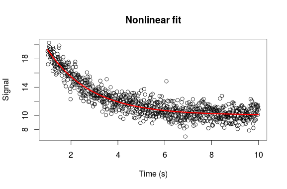
The Resulting Figure with R

rfit

And Finally with Octave


%Create x and y values
xdata = linspace(0, 10, 200);
ydata = 10 + 15.*exp(-xdata / 2) + randn(1, length(xdata));

%Define the exponential model
my_fun = @(p) sum((ydata- (p(1) + p(2).*exp(-xdata / p(3)))).^2);

%Function to evaluate the model. In this case we need to provide the error
%funtion: error sum of squares
fun_eval = @(p, t) p(1) + p(2).*exp(-t / p(3));

%Inital guesses
p0 = [min(ydata), max(ydata) - min(ydata), xdata(end) / 3]

%Nonlinear fit
result = fminsearch(my_fun, p0);

plot(xdata, ydata, 'k.')
hold on
plot(xdata, fun_eval(result, xdata), 'r')
xlabel('Time (s)')
ylabel('Signal')

The Respective Figure

octfit


PSD estimation of a RRi serie with Python

The new release o Scipy comes with the  modified periodogram method called Welch’s Periodogram. It is very similar to the pwelch function provided by Matlab and you’ll find it in scipy.signal.

Because some indices of heart rate variability are calculated in the frequency domain we first need to estimate the power spectral density (PSD) of the respective RRi signal. The welch function from scipy.signal allows you to choose the size of the segments, choose the overlap size and the window function (hanning, hamming,kaiser etc). It also provides two types of detrend methods: constant and linear. Although the welch function from scipy module is quite similar to the pwelch from Matlab, it does not calculates the Confidence Interval, which is a very important parameter, once RRi signals are stochastic.
So, in this post I’ll show how to estimate the PSD of a given RRi signal, calculate the 95% Confidence Interval of the respective PSD and then calculate its area under the curve: Very Low Frequency (VLF), Low Frequency (LF) and High Frequency (HF). The code will be written in Python with some parallel comparison to the Matlab pwelch function.

To implement this script we need just some functions from numpy and scipy:

from  numpy import cumsum, interp, arange
from scipy.signal import welch
from scipy.interpolate import splrep, splev

Then we need to load a RRi signal. In this example we’ll open a text file with the RRi values in a single column.

#Open RRi file
rri = [int(rri.strip())
       for rri in open('filename.txt') if rri.strip()]

tachogram

From the RRi values we need to create a time array. If your RRi values are in milliseconds you have to divide it by 1000.0, because later we’ll interpolate the RRi signal in 4 Hz.

#Create time array
# Divide by 1000.0 if RRi are in miliseconds.
t = cumsum(rri) / 1000.0 
#Force the time array to start from zero.
t -= t[0]

Because RRi are unevenly spaced we must interpolate it for accurate PSD estimation. In this case we’ll use the cubic spline interpolation.

#Create evenly spaced time array (4Hz).

#After the creation of a evenly spaced time
#array we are able to interpolate the RRi signal.
tx = arange(t[0], t[-1], 1.0 / 4.0)
tck = splrep(t, rri, s=0)
rrix = splev(tx, tck, der=0)

And Finally the PSD estimation with the non parametric Welch’s Method. As you can see here, the function provided by scipy for welch periodogam estimation look very similar to Matlab.

The Welch periodogram is an adaptation of the Bartlett method, which uses windows and data segmentation with overlap. The idea of the windows is to reduce the spectral leakage resulting in a decrease in spectral bias. With the overlaps more estimatives are made, so when all estimatives are averaged the spectral variance decreases.

Let’s consider a signal with N samples x[0],...,x[N-1]. The N samples signal is divided in P segments of D samples each with a shift S between adjacents segments. This way, the number of estimates are P, which is the integer part of (N-D)/S + 1.

The Welch periodogram can be calculated using the following equations.

\widetilde{P}_{xx}^{(p)}(f) = \frac{1}{UDT}|X^{(p)}(f)|^{2}

where X^{(p)}(f) is the discrete Fourier Transform of the pth segment:

X^{(p)}(f) = T \sum\limits_{n=0}^{D-1} x^{(p)}[n]e^{-j2 \pi fnT}

and U is the discrete window energy:

U= \frac{1}{D} \sum\limits_{n=0}^{D-1} w^2[n]

using a hanning window with 256 points its discrete energy is ~= 0.373.

Finally, averaging all P estimates we have the Welch’s periodogram:

\widetilde{P}_{xx}(f) = \frac{1}{P} \sum\limits_{p=0}^{P-1} \widetilde{P}_{xx}^{(p)}(f)

#PSD esitmation with hanning window, 256 points each segment with 50% overlap.
Fxx, Pxx = welch(x=rrix, fs=4.0, window="hanning",
                 nperseg=256, noverlap=128,
                 detrend="linear")

When we use pwelch in Matlab it’s possible to give two other parameters to this function: a string ‘ConfidenceLevel’ and the probability of the confidence interval. Giving these extra arguments a thirth output is returned:

[Pxx, Fxx, Pxxc] = pwelch(signal, window(segment),...
                           overlap, nfft, fs)

The Pxxc contains the 95% probability confidence interval of the PSD.

The welch function provided in scipy do not support theses argurments to calculate the confidence interval, but we can do it with few more lines of code using the chi2 function from scipy.stats

We can calculate the confidence interval of the actual PSD using a chi-square relationship. Given the estimate, the actual PSD lies between the limits with a desired probability. These relationship can described as follows:

\frac{\widetilde{P}_{xx}(f)}{\sigma^2P_k} \Longrightarrow \frac{\chi_ v^2}{2}

With these relation we can say that the confidence interval for the true Pxx is then:

\frac{2}{\chi_v^2(p/2)} \widetilde{P}_{xx}(f) \leq P_{xx} \leq \frac{2}{\chi_v^2(1 - p/2)} \widetilde{P}_{xx}(f)

where v is the degree of freedom and its equal to P (number of estimates) and p is the desired significance (p=0.05 for the 95% confidence interval). So to calculate the confidence interval of the PSD we’ll use the Percent Point Function of the chi-square with p = 0.05.

from scipy.stats import chi2

probability = 0.95

#P is the number of estimates in welch function
#and also the degree of freedom.
alfa = 1 - probability
v = 2 * P
c = chi2.ppf([1 - alfa / 2, alfa / 2], v)
c = v / c
Pxxc_lower = Pxx * c[0]
Pxxc_upper = Pxx * c[1]

psd

With our PSD we can now calculate the area under the curve from 0-0.04 Hz to estimate VLF, 0.04-0.15 to LF and 0.15-0.4 for HF. We’ll create a function called psd_auc that receives Fxx, Pxx and the frequency interval of each paramter. This function calculates the AUC with the sum of the respective PSD values multiplied by de frequency resolution:

\sum PSD(f)df

from numpy import logical_and

def psdauc(Fxx, Pxx, vlf=0.04, lf = 0.15, hf = 0.4):
    df = Fxx[1] - Fxx[0]
    vlf = sum(Pxx(Fxx <=  vlf)) * df
    lf = sum(Pxx[logical_and(Fxx >= vlf, Fxx < lf)]) * df
    hf = sum(Pxx[logical_and(Fxx >= lf, Fxx < hf)]) * df
    return vlf, lf, hf

You can find the code of this post here