Sometimes in biological research we want to extract some parameter from a dynamical system, such as: response of blood pressure in function of a drug dose, growth of bacterial population over time or the recovery of the heart rate after a exercise session. One way to get some informations about these processes is to fit a model which has some parameters that can explain the behavior of the data. The parametrization of a set of values can be taken from a linear or nonlinear models. The most common method to fit all types of models is the least squares method (LSM) which finds the minimum of the error curve.
In this post I’m gonna fit a theoretical curve with some noise added to a first order exponential model using the leastq function provided by scipy.optimize, which is the optimization module from Scipy. I’ll also make the same fit with R and Octave, using the nls and fminsearch functions, respectively.
The first order exponential model can be described as fallows:
Where is the asymptotic value as t goes to infinity;
is the gain and
is the time constant
Code for nonlinear fit with Python
import numpy as np
import matplotlib.pyplot as plt
from scipy.optimize import leastsq

#Create the x and y values
xdata = np.linspace(0, 10, 200)
ydata = 10 + 15 * np.exp(-xdata / 2) + np.random.randn(len(xdata))


#Define the exponential model
def my_fun(par, t, y):
    err = y - (par[0] + par[1] * np.exp(-t / par[2]))
    return err


#Function to evaluate the model
def fun_eval(par, t):
    return par[0] + par[1] * np.exp(-t / par[2])

#Initial guesses
p0 = [min(ydata), max(ydata) - min(ydata), xdata[-3] / 3]

#Nonlinear fit
result = leastsq(my_fun, p0, args=(xdata, ydata))

#Plot the curves
plt.plot(xdata, ydata, 'k.')
plt.plot(xdata, fun_eval(result[0], xdata), 'r')
plt.xlabel("Time (s)")
plt.ylabel("Signal")
plt.show()
The Resulting Figure
 Using R
#Create the x and y values
xdata <- seq(1, 10, by=1 / 100)
ydata <- 10 + 15 * exp(-xdata / 2) + rnorm(length(xdata))

#Create a data frame
data_frame <- data.frame(xdata=xdata, ydata=ydata)

#Model
myfun <- function(time, b1, b2, b3){
    b1 + b2 * exp(-time / b3)
}

#Inital guesses
p0 <- list(b1=min(ydata), b2=max(ydata) - min(ydata),b3=tail(xdata, n=1) / 3)

#Nonlinear fit
result <- nls(ydata ~ myfun(xdata, b1, b2, b3), data=data_frame, start=p0)

#Plot the curves
plot(xdata, ydata, xlab="Time (s)", ylab="Signal")
lines(xdata, predict(result, list(xdata)), lwd=3, col="red")
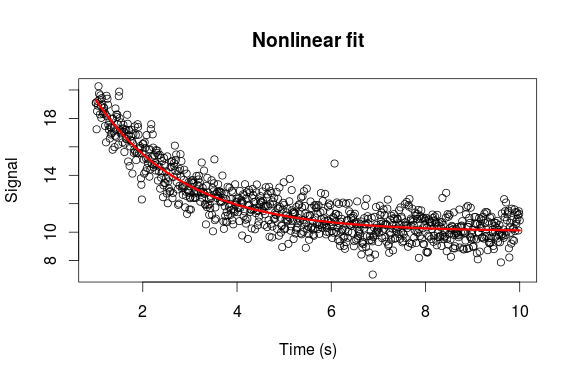
The Resulting Figure with R
And Finally with Octave
%Create x and y values
xdata = linspace(0, 10, 200);
ydata = 10 + 15.*exp(-xdata / 2) + randn(1, length(xdata));

%Define the exponential model
my_fun = @(p) sum((ydata- (p(1) + p(2).*exp(-xdata / p(3)))).^2);

%Function to evaluate the model. In this case we need to provide the error
%funtion: error sum of squares
fun_eval = @(p, t) p(1) + p(2).*exp(-t / p(3));

%Inital guesses
p0 = [min(ydata), max(ydata) - min(ydata), xdata(end) / 3]

%Nonlinear fit
result = fminsearch(my_fun, p0);

plot(xdata, ydata, 'k.')
hold on
plot(xdata, fun_eval(result, xdata), 'r')
xlabel('Time (s)')
ylabel('Signal')
The Respective Figure
